Calculate power for global and/or pairwise hypothesis tests of survival data with support over a range of data structures from different experimental designs. Power calculations can be made to account for inter-tank variation using a mixed cox proportional hazards model (set argument model = "coxph_glmm"). Additionally, power calculations can account for the multiplicity of pairwise comparisons using pairwise_corr. Users can compare power across different experimental designs by specifying each as a list element in Surv_Simul(). A brief tutorial is written in Examples to guide the user on how to use Surv_Power() to calculate power under various scenarios.
Usage
Surv_Power(
  simul_db = simul_db_ex,
  global_test = "logrank",
  model = NULL,
  pairwise_test = "logrank",
  pairwise_corr = c("none", "BH"),
  prog_show = TRUE,
  data_out = TRUE,
  plot_out = TRUE,
  plot_lines = FALSE,
  xlab = "List Element #",
  xnames = NULL,
  plot_save = TRUE
)
Arguments
- simul_db
An output from
Surv_Simul()which includes the survival dataframe simulated with the desired experimental design parameters.- global_test
A character vector representing the method(s) to use for global hypothesis testing of significance of treatment. Methods available are: "logrank", "wald", "score", "LRT". "logrank" represents the global logrank test of significance. The latter three methods are standard global hypothesis testing methods for models. They are only available when the argument
modelis specified (i.e. not NULL). "wald" represents the Wald Chisquare Test which assesses whether model parameters (log(hazard ratios)) jointly are significantly different from 0 (i.e. HRs ≠ 1). Wald test can be done for various cox-proportional hazard models that could be relevant to our studies (glm, glmm, and gee). Due to its broad applicability, while also producing practically the same p-value most of the time compared to the other model tests, "wald" is the recommended option of the three. "score" represents the Lagrange multiplier or Score test. 'LRT' represents the likelihood ratio test. Defaults to "logrank" for now due to its ubiquity of use.- model
A character vector representing the model(s) to fit for hypothesis testing. Models available are: "coxph_glm" and "coxph_glmm" ("cox_gee" may be supported upon request, omitted for reasons not discussed here). "coxph_glm" represents the standard cox proportional hazard model fitted using
survival::coxph()with Trt.ID as a fixed factor. "coxph_glmm" represents the mixed cox proportional hazard model fitted usingcoxme::coxme()with Trt.ID as a fixed factor and Tank.ID as a random factor to account for inter-tank variation. Defaults to NULL where no model is fitted for hypothesis testing.- pairwise_test
A character vector representing the method(s) used for pairwise hypothesis tests. Use "logrank" to calculate power for logrank tests comparing different treatments. Use "EMM" to calculate power using Estimated Marginal Means based on model estimates (from 'coxph_glm' and/or 'coxph_glmm'). Defaults to "logrank".
- pairwise_corr
A character vector representing the method(s) used to adjust p-values for multiplicity of pairwise comparisons. For clarification, this affects the power of the pairwise comparisons. Methods available are: "tukey", "holm", "hochberg", "hommel", "bonferroni", "BH", "BY", and "none". Under Details (yet to be finished), I discuss the common categories of adjustment methods and provided a recommendation for "BH". Defaults to c("none", "BH").
- prog_show
Whether to display the progress of
Surv_Power()by printing the number of sample sets with p-values calculated. Defaults to TRUE.- data_out
Whether to output dataframes containing the power of global and/or pairwise hypothesis tests. Defaults to TRUE.
- plot_out
Whether to output plots illustrating the power of global and/or pairwise hypothesis tests. Defaults to TRUE.
- plot_lines
Whether to plot lines connecting points of the same hypothesis test in the plot output. Defaults to TRUE.
- xlab
A string representing the x-axis title. Defaults to "List Element #".
- xnames
A character vector of names for x-axis labels. Defaults to NULL where names are the list element numbers from
Surv_Simul().- plot_save
Whether to save plots as a .tiff in the working directory. Defaults to TRUE.
Value
Outputs a list containing any of the following four items depending on input arguments:
When
global_test ≠ NULLanddata_out = TRUE, outputs a dataframe namedpower_glob_dbcontaining power values calculated for global hypothesis tests. The dataframe consists of six columns:modelThe type of model being evaluated in power calculations global_testThe global hypothesis test being evaluated powerThe percentage of p-values below 0.05, i.e. power power_seStandard error for percentages sample_sets_nNumber of sample sets used in calculating power list_element_numThe list element number associated with the power value calculated When
global_test ≠ NULLandplot_out = TRUE, a plot showing power values for global hypothesis test. Plot corresponds topower_glob_db.When
pairwise_test ≠ NULLanddata_out = TRUE, outputs a dataframe namedpower_pair_dbcontaining power values for pairwise hypothesis tests. The dataframe consists of eight columns:pairThe treatment groups to be compared modelThe type of model being evaluated in power calculations pairwise_testThe type of pairwise_test being evaluated pairwise_corrThe method of p-value correction/adjustments for paiwrise comparisons powerThe percentage of p-values below 0.05, i.e. power power_seStandard error for percentages sample_sets_nNumber of sample sets used in calculating power list_element_numThe list element number associated with the power value calculated When
pairwise_test ≠ NULLandplot_out = TRUE, a plot showing power values across list elements. Plot corresponds topower_pair_db.
See also
Link for web documentation.
Examples
# Below is a tutorial on how to calculate power using Surv_Power(). The function
# calculates power as a percentage of positive (p < 0.05) test conducted on simulated
# datasets. Hence, the first step is simulating the data
# A past data is retrieved for simulating future datasets:
data(haz_db_ex)
haz_db_ex = haz_db_ex[haz_db_ex$Trt.ID == "A",] # filter for control fish
head(haz_db_ex, n = 5)
#> Trt.ID Hazard Time
#> 1 A 1.098677e-10 0.5
#> 2 A 2.321493e-10 1.5
#> 3 A 4.905294e-10 2.5
#> 4 A 1.036484e-09 3.5
#> 5 A 2.190081e-09 4.5
# As may be clear from the above, we are using the past data's hazard curve properties.
# NOTE: Whether the shape of the hazard curve repeats in the future study only matters
# to the accuracy of the power calculation when the future study involves fish being
# dropped (e.g. due to sampling).
# To begin simulating, input the past data to Surv_Simul() with the supposed future
# experiment parameters:
surv_sim_db_ex1 = Surv_Simul(haz_db = haz_db_ex,
fish_num_per_tank = 100,
tank_num_per_trt = 4,
treatments_hr = c(1, 0.7, 0.5),
logHR_sd_intertank = 0,
n_sim = 500,
prog_show = FALSE, #omit progress bar for cleaner output
plot_out = FALSE) #omit plotting for efficiency/speed
#> [1] "Time elapsed: 00:00:02 (hh:mm:ss)"
# Above, we simulated 500 datasets with each having 400 fish per treatment and three
# treatments total with hazard ratios of 1, 0.7, and 0.5 relative to 'haz_db_ex.'
# Next, the simulated data can be supplied to Surv_Power() to calculate power. Below,
# power is calculated for the logrank test:
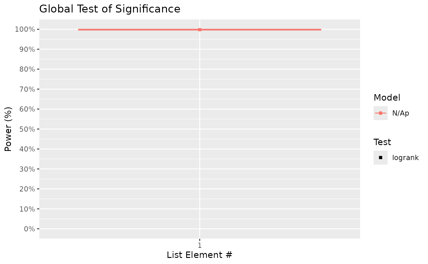
Surv_Power(simul_db = surv_sim_db_ex1,
global_test = "logrank",
pairwise_test = "logrank",
pairwise_corr = "none",
prog_show = FALSE,
data_out = FALSE) # remove data output for brevity
#> [1] "Time elapsed: 00:00:11 (hh:mm:ss)"
#> $power_global_plot
 #>
#> $power_pairwise_plot
#>
#> $power_pairwise_plot
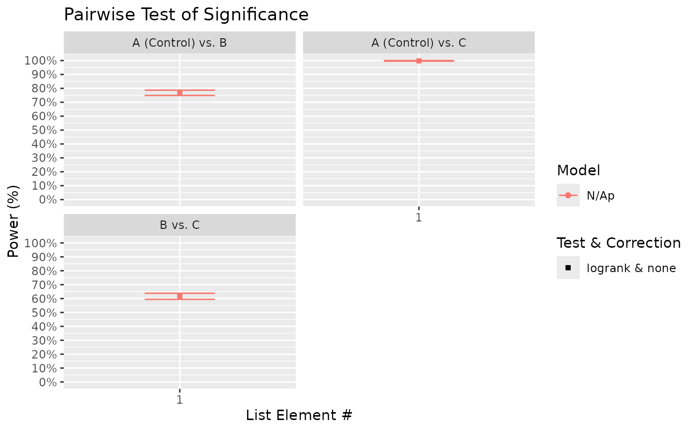 #>
# From the above, we can see that there is a high probability of detecting significance
# of treatment using the global test. On the other hand, power to detect differences
# between treatment B (HR = 0.7 relative to control) and C (HR = 0.5) is ~ 60%.
# Notably, the presented power for pairwise comparisons uses unadjusted p-values.
# If there is a need to adjust p-values to provide a guarantee for, for example, the
# false discovery rate, then supply the chosen FDR method(s) (e.g. "BH") to the
# 'pairwise_corr' argument:
Surv_Power(simul_db = surv_sim_db_ex1,
global_test = "logrank",
pairwise_test = "logrank",
pairwise_corr = c("none", "BH"),
prog_show = FALSE,
data_out = FALSE)
#> [1] "Time elapsed: 00:00:16 (hh:mm:ss)"
#> $power_global_plot
#>
# From the above, we can see that there is a high probability of detecting significance
# of treatment using the global test. On the other hand, power to detect differences
# between treatment B (HR = 0.7 relative to control) and C (HR = 0.5) is ~ 60%.
# Notably, the presented power for pairwise comparisons uses unadjusted p-values.
# If there is a need to adjust p-values to provide a guarantee for, for example, the
# false discovery rate, then supply the chosen FDR method(s) (e.g. "BH") to the
# 'pairwise_corr' argument:
Surv_Power(simul_db = surv_sim_db_ex1,
global_test = "logrank",
pairwise_test = "logrank",
pairwise_corr = c("none", "BH"),
prog_show = FALSE,
data_out = FALSE)
#> [1] "Time elapsed: 00:00:16 (hh:mm:ss)"
#> $power_global_plot
 #>
#> $power_pairwise_plot
#>
#> $power_pairwise_plot
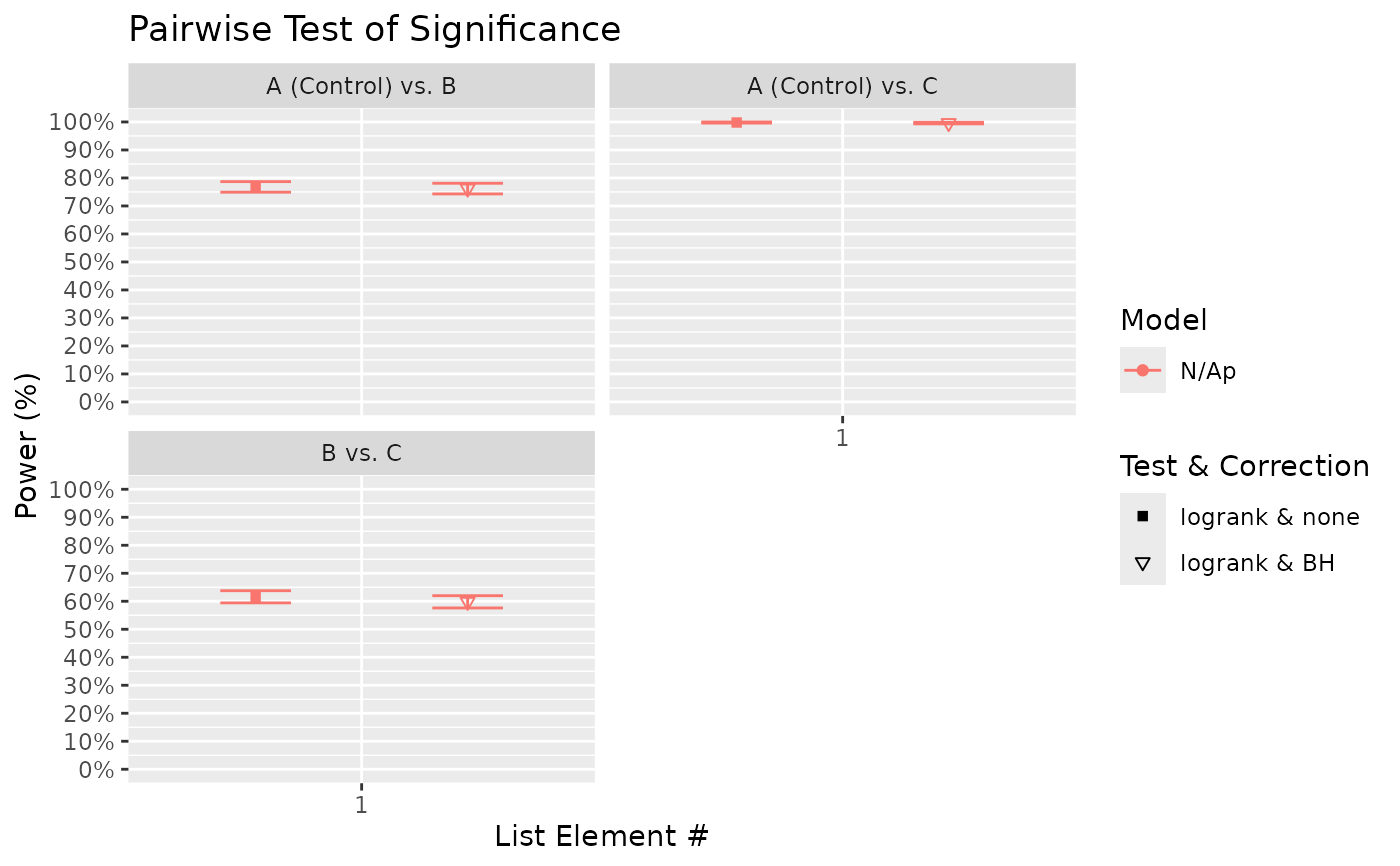 #>
# By default, FDR adjustment methods "control" or limit the false discovery rate to 5%;
# true FDR would be lower.
# If for some reason there is a need to control for family-wise error rate due to a
# desire to conclude at the family-level (already achievable via global test), then p
# values can be adjusted using FWER methods (e.g. "bonferroni", "tukey"). Notably, due
# to the correlation between pairwise tests, the tukey method is possible and is more
# powerful than bonferroni. The tukey option is available if a model is specified:
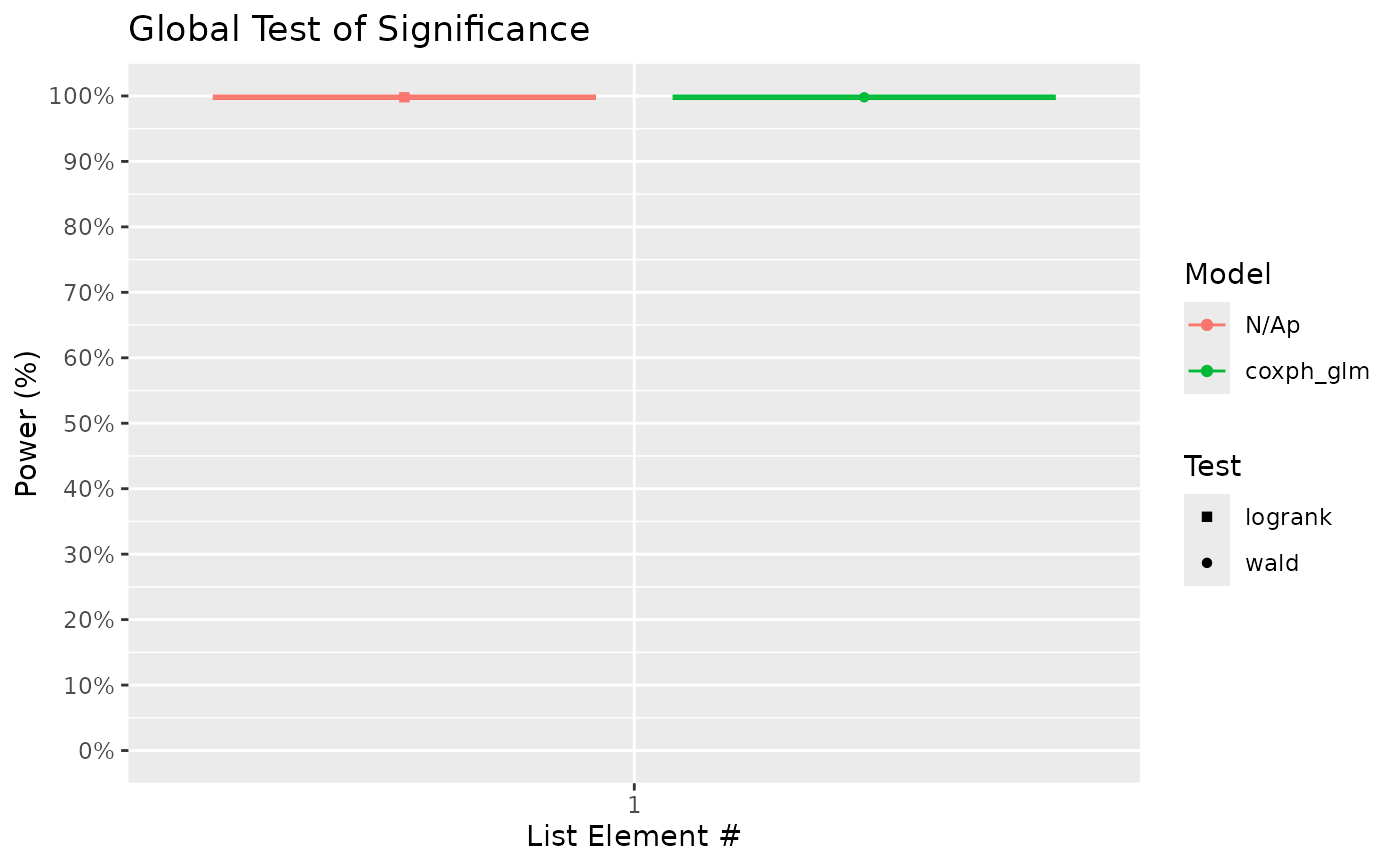
Surv_Power(simul_db = surv_sim_db_ex1,
model = "coxph_glm",
global_test = c("logrank", "wald"),
pairwise_test = c("logrank", "EMM"),
pairwise_corr = c("none", "tukey", "bonferroni"),
prog_show = FALSE,
data_out = FALSE)
#> [1] "NOTE: Tukey pairwise correction is not available for log-rank tests. No power value is returned for such a combination of test and correction."
#> [1] "Time elapsed: 00:01:22 (hh:mm:ss)"
#> $power_global_plot
#>
# By default, FDR adjustment methods "control" or limit the false discovery rate to 5%;
# true FDR would be lower.
# If for some reason there is a need to control for family-wise error rate due to a
# desire to conclude at the family-level (already achievable via global test), then p
# values can be adjusted using FWER methods (e.g. "bonferroni", "tukey"). Notably, due
# to the correlation between pairwise tests, the tukey method is possible and is more
# powerful than bonferroni. The tukey option is available if a model is specified:
Surv_Power(simul_db = surv_sim_db_ex1,
model = "coxph_glm",
global_test = c("logrank", "wald"),
pairwise_test = c("logrank", "EMM"),
pairwise_corr = c("none", "tukey", "bonferroni"),
prog_show = FALSE,
data_out = FALSE)
#> [1] "NOTE: Tukey pairwise correction is not available for log-rank tests. No power value is returned for such a combination of test and correction."
#> [1] "Time elapsed: 00:01:22 (hh:mm:ss)"
#> $power_global_plot
 #>
#> $power_pairwise_plot
#>
#> $power_pairwise_plot
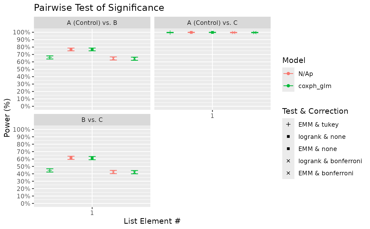 #>
# Based on the pairwise plot above, it seems that the tukey method is only marginally
# more powerful in this case compared to bonferroni. The model used above was the cox
# proportional hazards model. The global test option "wald" corresponds to a wald
# chi-square test of the significance of treatment as a model factor. The pairwise
# test option "EMM" corresponds to treatment comparisons using model estimated
# marginal means. Notably, the model methods appear to produced similar result to the
# logrank test, at least in this example.
# More sophisticated models may be fitted to account for tank variation if any was
# introduced in the simulation process as below:
surv_sim_db_ex2 = Surv_Simul(haz_db = haz_db_ex,
fish_num_per_tank = 100,
tank_num_per_trt = 6,
treatments_hr = c(1, 1, 0.7),
logHR_sd_intertank = 0.2,
n_sim = 500,
prog_show = FALSE,
plot_out = FALSE)
#> [1] "Time elapsed: 00:00:02 (hh:mm:ss)"
# To calculate power considering the tank variation, we fit a mixed model (coxph_glmm):
Surv_Power(simul_db = surv_sim_db_ex2,
model = "coxph_glmm",
global_test = c("logrank", "wald"),
pairwise_test = c("logrank", "EMM"),
pairwise_corr = c("none"),
prog_show = FALSE,
data_out = FALSE)
#> [1] "Time elapsed: 00:01:19 (hh:mm:ss)"
#> $power_global_plot
#>
# Based on the pairwise plot above, it seems that the tukey method is only marginally
# more powerful in this case compared to bonferroni. The model used above was the cox
# proportional hazards model. The global test option "wald" corresponds to a wald
# chi-square test of the significance of treatment as a model factor. The pairwise
# test option "EMM" corresponds to treatment comparisons using model estimated
# marginal means. Notably, the model methods appear to produced similar result to the
# logrank test, at least in this example.
# More sophisticated models may be fitted to account for tank variation if any was
# introduced in the simulation process as below:
surv_sim_db_ex2 = Surv_Simul(haz_db = haz_db_ex,
fish_num_per_tank = 100,
tank_num_per_trt = 6,
treatments_hr = c(1, 1, 0.7),
logHR_sd_intertank = 0.2,
n_sim = 500,
prog_show = FALSE,
plot_out = FALSE)
#> [1] "Time elapsed: 00:00:02 (hh:mm:ss)"
# To calculate power considering the tank variation, we fit a mixed model (coxph_glmm):
Surv_Power(simul_db = surv_sim_db_ex2,
model = "coxph_glmm",
global_test = c("logrank", "wald"),
pairwise_test = c("logrank", "EMM"),
pairwise_corr = c("none"),
prog_show = FALSE,
data_out = FALSE)
#> [1] "Time elapsed: 00:01:19 (hh:mm:ss)"
#> $power_global_plot
 #>
#> $power_pairwise_plot
#>
#> $power_pairwise_plot
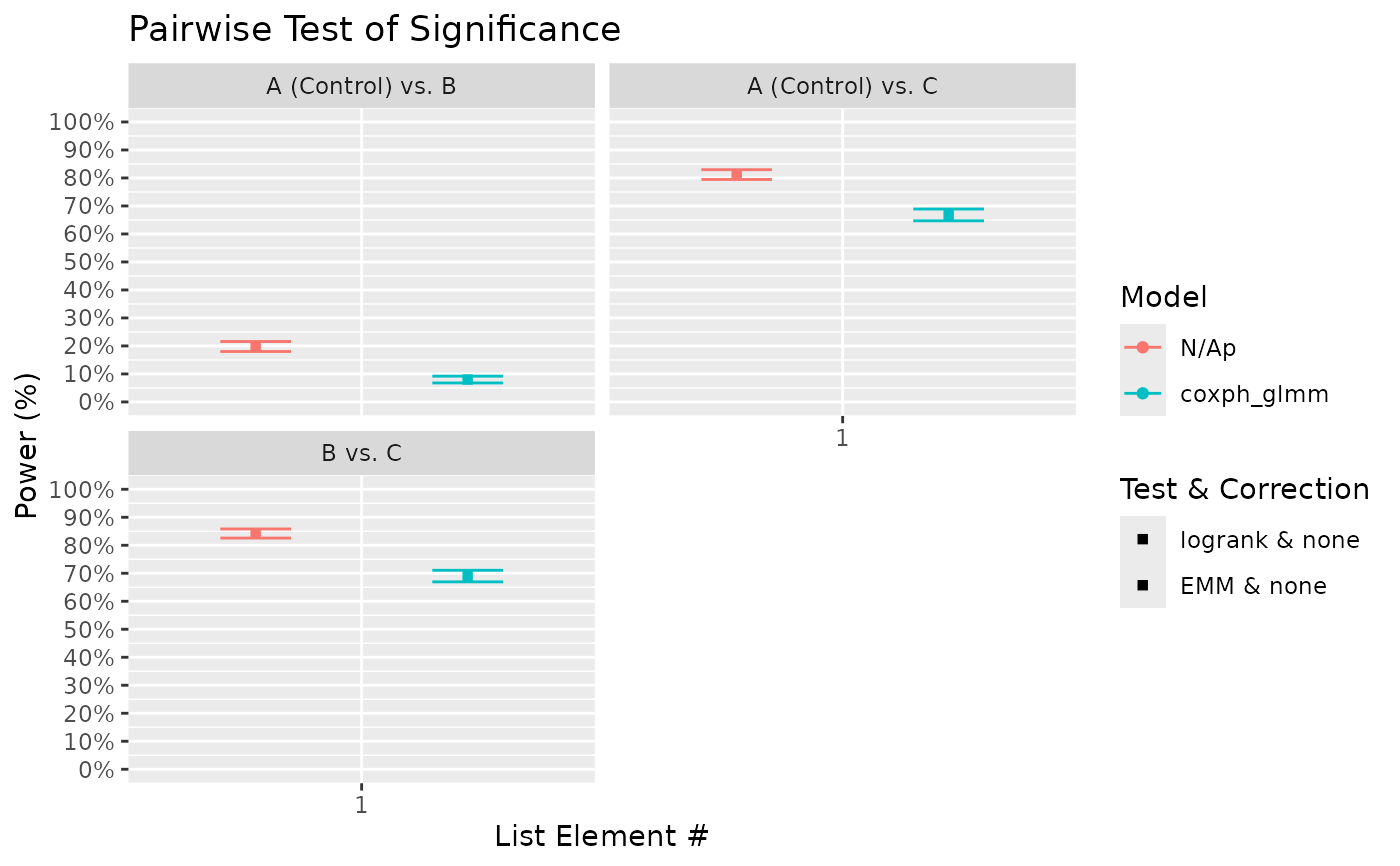 #>
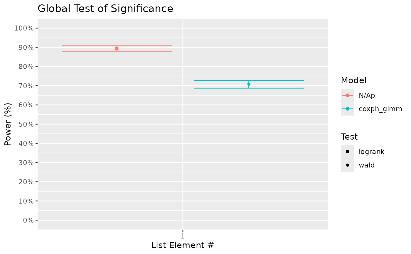
# The above results show a property of the test that accounted for tank variation;
# it is weaker than the one that does not (logrank test) given the data has tank
# variability. However, this is for a reason. If you look into the positive rate of
# the test comparing Control vs Trt. B (where true HR = 1), it only slightly above 5%
# for the mixed model (a real bias for reasons not discussed here). This result is
# roughly consistent with the acclaimed alpha or false positive rate of 0.05. In
# contrast, the false positive rate for logrank test is much higher at ~20%.
## VARYING EXPERIMENTAL CONDITIONS
# As a precautionary measure, it may be important to study power under various scenarios
# (e.g. increasing or decreasing strength of pathogen challenge). To do this, specify
# each scenario as separate elements of a list in an argument of Surv_Simul():
HR_vec = c(1, 0.7, 0.5)
HR_list = list(1.5 * HR_vec, # strong challenge
1.0 * HR_vec, # medium challenge
0.5 * HR_vec) # weak challenge
surv_sim_db_ex3 = Surv_Simul(haz_db = haz_db_ex,
fish_num_per_tank = 100,
tank_num_per_trt = 4,
treatments_hr = HR_list,
logHR_sd_intertank = 0,
n_sim = 500,
prog_show = FALSE,
plot_out = FALSE)
#> [1] "Time elapsed: 00:00:05 (hh:mm:ss)"
# Next, calculate and compare power across scenarios:
Surv_Power(simul_db = surv_sim_db_ex3,
global_test = "logrank",
pairwise_test = "logrank",
pairwise_corr = "none",
prog_show = FALSE,
data_out = FALSE,
xlab = "Challenge Strength",
xnames = c("Strong", "Medium", "Weak"))
#> [1] "Time elapsed: 00:00:30 (hh:mm:ss)"
#> $power_global_plot
#>
# The above results show a property of the test that accounted for tank variation;
# it is weaker than the one that does not (logrank test) given the data has tank
# variability. However, this is for a reason. If you look into the positive rate of
# the test comparing Control vs Trt. B (where true HR = 1), it only slightly above 5%
# for the mixed model (a real bias for reasons not discussed here). This result is
# roughly consistent with the acclaimed alpha or false positive rate of 0.05. In
# contrast, the false positive rate for logrank test is much higher at ~20%.
## VARYING EXPERIMENTAL CONDITIONS
# As a precautionary measure, it may be important to study power under various scenarios
# (e.g. increasing or decreasing strength of pathogen challenge). To do this, specify
# each scenario as separate elements of a list in an argument of Surv_Simul():
HR_vec = c(1, 0.7, 0.5)
HR_list = list(1.5 * HR_vec, # strong challenge
1.0 * HR_vec, # medium challenge
0.5 * HR_vec) # weak challenge
surv_sim_db_ex3 = Surv_Simul(haz_db = haz_db_ex,
fish_num_per_tank = 100,
tank_num_per_trt = 4,
treatments_hr = HR_list,
logHR_sd_intertank = 0,
n_sim = 500,
prog_show = FALSE,
plot_out = FALSE)
#> [1] "Time elapsed: 00:00:05 (hh:mm:ss)"
# Next, calculate and compare power across scenarios:
Surv_Power(simul_db = surv_sim_db_ex3,
global_test = "logrank",
pairwise_test = "logrank",
pairwise_corr = "none",
prog_show = FALSE,
data_out = FALSE,
xlab = "Challenge Strength",
xnames = c("Strong", "Medium", "Weak"))
#> [1] "Time elapsed: 00:00:30 (hh:mm:ss)"
#> $power_global_plot
 #>
#> $power_pairwise_plot
#>
#> $power_pairwise_plot
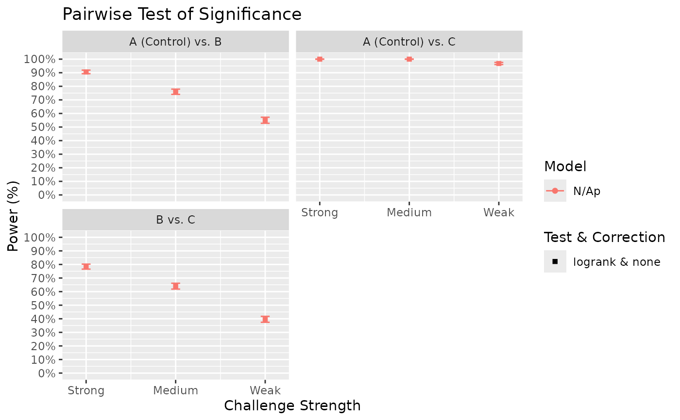 #>
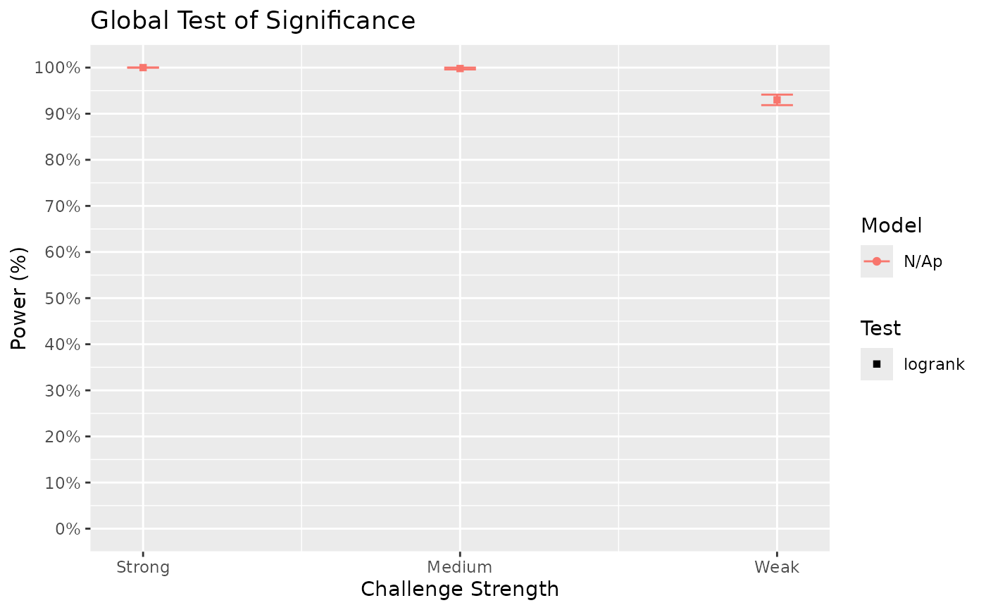
# The results show that power for the strong challenge model is generally high.
# However, for the weak challenge model, more sample size appears to be needed to
# achieve 80% power for some pairwise comparisons. We can investigate at what sample
# size would such power be achieved by specifying different sample sizes as separate
# list elements in Surv_Simul():
fish_num_vec = seq(from = 50, to = 200, by = 30)
fish_num_vec
#> [1] 50 80 110 140 170 200
fish_num_list = as.list(fish_num_vec) # convert vector elements to list elements
# Simulate the different experimental conditions:
surv_sim_db_ex4 = Surv_Simul(haz_db = haz_db_ex,
fish_num_per_tank = fish_num_list,
tank_num_per_trt = 4,
treatments_hr = c(1, 0.7, 0.5) * 0.5,
logHR_sd_intertank = 0,
n_sim = 500,
prog_show = FALSE,
plot_out = FALSE)
#> [1] "Time elapsed: 00:00:14 (hh:mm:ss)"
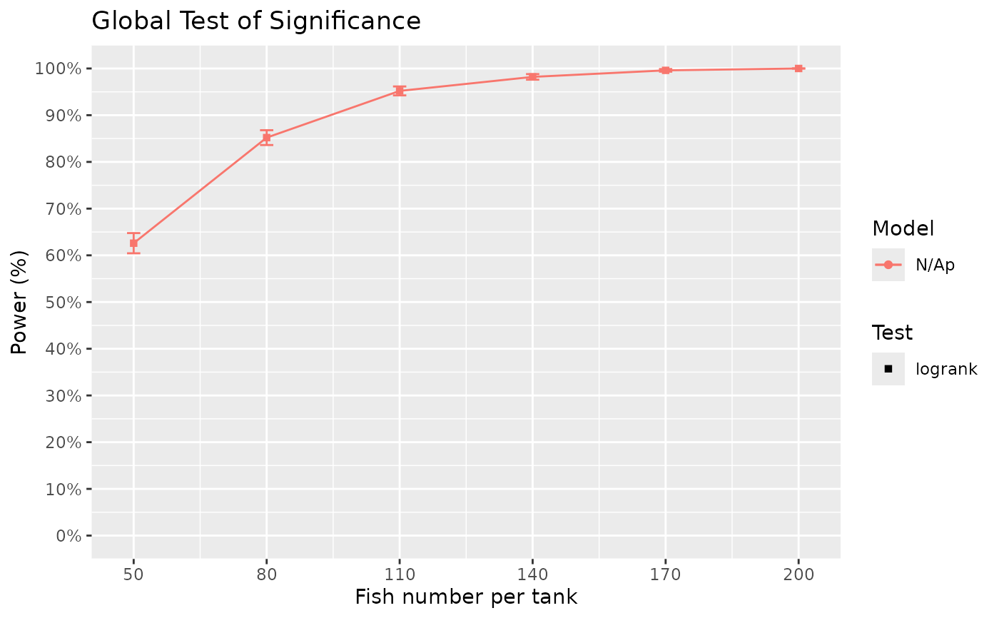
# Compare power across sample sizes:
Surv_Power(simul_db = surv_sim_db_ex4,
global_test = "logrank",
pairwise_test = "logrank",
pairwise_corr = "none",
prog_show = FALSE,
data_out = FALSE,
xlab = "Fish number per tank",
xnames = fish_num_vec,
plot_lines = TRUE)
#> [1] "Time elapsed: 00:01:03 (hh:mm:ss)"
#> $power_global_plot
#>
# The results show that power for the strong challenge model is generally high.
# However, for the weak challenge model, more sample size appears to be needed to
# achieve 80% power for some pairwise comparisons. We can investigate at what sample
# size would such power be achieved by specifying different sample sizes as separate
# list elements in Surv_Simul():
fish_num_vec = seq(from = 50, to = 200, by = 30)
fish_num_vec
#> [1] 50 80 110 140 170 200
fish_num_list = as.list(fish_num_vec) # convert vector elements to list elements
# Simulate the different experimental conditions:
surv_sim_db_ex4 = Surv_Simul(haz_db = haz_db_ex,
fish_num_per_tank = fish_num_list,
tank_num_per_trt = 4,
treatments_hr = c(1, 0.7, 0.5) * 0.5,
logHR_sd_intertank = 0,
n_sim = 500,
prog_show = FALSE,
plot_out = FALSE)
#> [1] "Time elapsed: 00:00:14 (hh:mm:ss)"
# Compare power across sample sizes:
Surv_Power(simul_db = surv_sim_db_ex4,
global_test = "logrank",
pairwise_test = "logrank",
pairwise_corr = "none",
prog_show = FALSE,
data_out = FALSE,
xlab = "Fish number per tank",
xnames = fish_num_vec,
plot_lines = TRUE)
#> [1] "Time elapsed: 00:01:03 (hh:mm:ss)"
#> $power_global_plot
 #>
#> $power_pairwise_plot
#>
#> $power_pairwise_plot
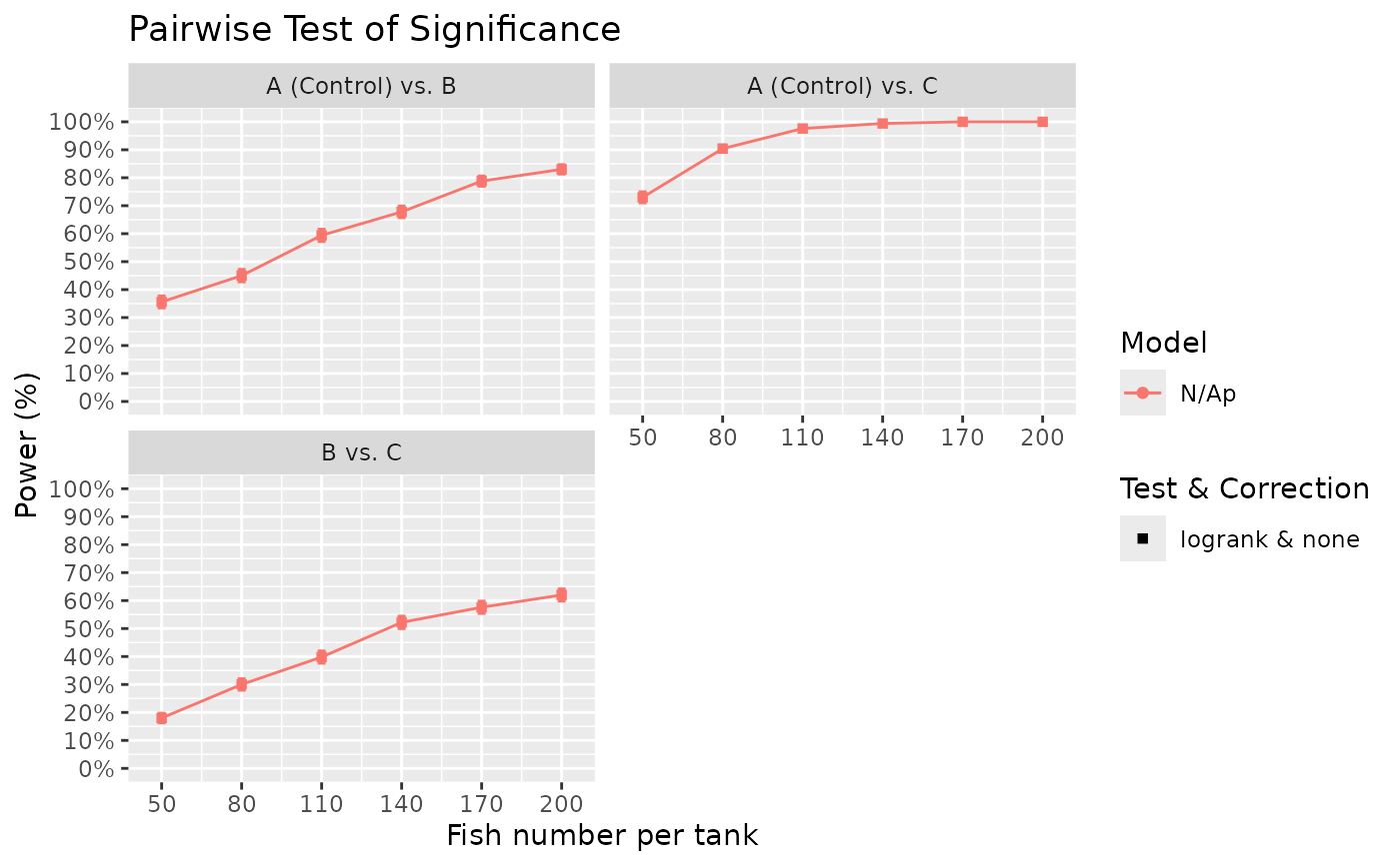 #>
# The results showed that even an increase in sample size (from 100 to 200) result in
# only modest gains in power for comparisons B to C. Perhaps a possible future action
# then is to ensure the challenge is medium to strong by having higher salinity for
# example. The above examples show some possible use case of Surv_Power(), but other
# cases can be simulated to understand power in various scenarios. I hope this tool
# can help you calculate power for your specific needs!
#>
# The results showed that even an increase in sample size (from 100 to 200) result in
# only modest gains in power for comparisons B to C. Perhaps a possible future action
# then is to ensure the challenge is medium to strong by having higher salinity for
# example. The above examples show some possible use case of Surv_Power(), but other
# cases can be simulated to understand power in various scenarios. I hope this tool
# can help you calculate power for your specific needs!