Get Started!

Welcome to the documentation of the R package safuncs! This package is designed to assist you in the analysis of your biological data (e.g. survival).

Below I wrote a short tutorial on how some of the core functions in safuncs can be used.

To get started, please install and load the package by running the following code:

remotes::install_github("sean4andrew/safuncs") # install package
library(safuncs) # load

Survival Analysis

At ONDA, survival data is often available to scientists initially in the form of rows of entries for every mortality observed. This data needs to be converted to a useful form for analysis in R or Prism. The function Surv_Gen() shortens the data transformation step to just one line of code! Below, I showcase its use.

Let us first examine the raw survival data we can get from our OneDrive mort excel file:

data(mort_db_ex) # load example data file
head(mort_db_ex, n = 5) # view first 5 rows of data
#>   Tank.ID Trt.ID TTE Status
#> 1      C1      B   0      1
#> 2      C6      B   4      1
#> 3      C6      B   7      1
#> 4      C1      B  19      1
#> 5      C8      D  19      1

The 2nd-rightmost column named TTE indicates the Time to Event, e.g. days post challenge, and the last column Status indicates the type of event (1 = death, 0 = sampled-out or survived). Missing from such a dataset are the rows representing surviving fish (Status = 0); these needs to be present for a proper survival analysis.

Introducing Surv_Gen()!

Obtain the proper survival data by simply inserting the mort database into Surv_Gen(). Provide a time (TTE) indicating until when other fish survived and the starting number of fish used per tank.

Surv_Gen(mort_db = mort_db_ex,
         starting_fish_count = 100, # per tank
         last_tte = 54)

Below is the output data’s bottom 5 rows which represent the generated survivors (Status = 0).

#>      Tank.ID Trt.ID TTE Status
#> 1196      C8      D  54      0
#> 1197      C8      D  54      0
#> 1198      C8      D  54      0
#> 1199      C8      D  54      0
#> 1200      C8      D  54      0

You also get some printout messages for verification purposes:

#> [1] "Your total number of tanks is: 12"
#> [1] "Your total number of treatment groups is: 4"
#> [1] "Your total number of fish in the output data is: 1200"

You can also specify tank-specific starting fish numbers using a dataframe as input to starting_fish_count!

# reduce example data to simplify the demonstration
mort_db_ex2 = mort_db_ex[mort_db_ex$Tank.ID %in% c("C01", "C02", "C03"),]

# apply Surv_Gen()!
Surv_Gen(mort_db = mort_db_ex2,
         starting_fish_count = data.frame(Trt.ID = c("B", "A", "C"), # a vector of treatment groups for the specified tanks
                                          Tank.ID = c("C1", "C2", "C3"), # a vector with ALL tanks in the study
                                          starting_fish_count = c(100, 100, 50)), # a vector of fish numbers in same order as Tank.IDs
         last_tte = 54)

With a short R script as shown, you can quickly regenerate survival data whenever there is a slight change in the mort database; perhaps from day-to-day or after corrections.

For those wanting to use the generated survival data in prism, set the argument output_prism = TRUE in Surv_Gen() to save a prism-ready csv. in your working directory. If you want starting and ending dates in the Prism output, input a starting date into the argument output_prism_date, as shown:

Surv_Gen(mort_db = mort_db_ex,
         starting_fish_count = 100, # per tank
         last_tte = 54,
         output_prism = TRUE,
         output_prism_date = "08-Aug-2024")

Once the complete survival data has been obtained, plots can be easily generated using Surv_Plots()!

data(surv_db_ex) # load example complete survival data

Surv_Plots(surv_db_ex, # plot the survival curve and hazard curve
           dailybin = FALSE) # recommended argument for good (large) sample size datasets
#> $Survival_Plot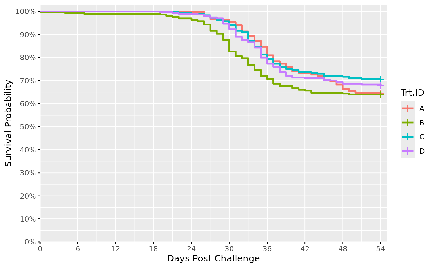

#> 
#> $Hazard_Plot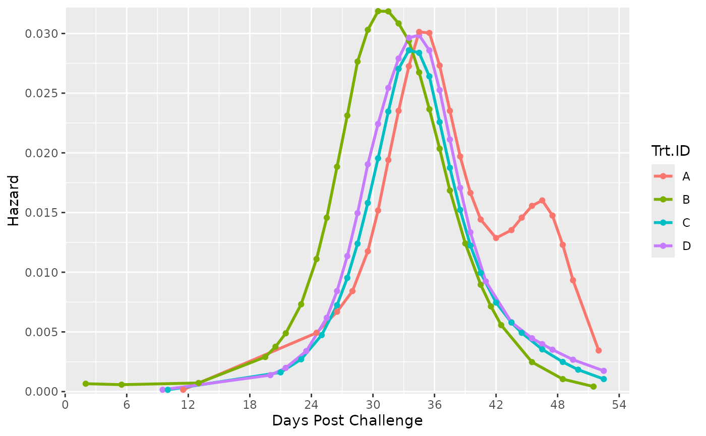

The plots save automatically to your working directory as a .tiff and in a power-point editable format (.pptx). Notably, Surv_Plots() accepts many more arguments that can influence the hazard plot in particular and needs tailoring for your specific experiment. For more details on these arguments, please see the functions’ documentation page.

############TO BE CONTINUED###########

Sean Andrew

2025-07-03

Survival Analysis