Produces a Kaplan-Meier Survival Plot and/or Hazard Time Plot from survival data. Each plot contains multiple curves for the different groups. Plots are saved by automatically to working directory as .tiff and .pptx.
Usage
Surv_Plots(
  surv_db,
  factor = "Trt.ID",
  xlim = NULL,
  xbreaks = NULL,
  xlab = "Days Post Challenge",
  ylim = c(0, 1.03),
  lambda = NULL,
  phi = NULL,
  dailybin = TRUE,
  plot = "both",
  colours = NULL,
  theme = "ggplot",
  haz_points = TRUE,
  data_out = FALSE,
  plot_save = TRUE,
  plot_prefix = "ONDA_XX",
  plot_dim = c(6, 4),
  legend_cols = NULL,
  linesize = 1
)
Arguments
- surv_db
A survival dataframe as described in Details.
- factor
A string representing the formula of factors (column names) which represent the structure of the plot. Accepts single to two factors with interactions; "Tank.ID * Trt.ID" creates curves for every tank and treatment combination, "Trt.ID - Tank.ID" does the same but distinguishes the curves by color across treatments and by linetype across tanks, while "Tank.ID | Trt.ID" creates curves for every tank faceted by treatment.
- xlim
A vector specifying the plots x-axis lower and upper limits, respectively.
- xbreaks
A number specifying the interval for every major tick in the x-axis.
- xlab
A string specifying the plot x-axis label. Defaults to "Days Post Challenge".
- ylim
A vector specifying the Survival Plot y-axis lower and upper limits, respectively. Defaults to c(0, 1) which indicates 0 to 100% Survival Probability, respectively.
- lambda
Smoothing value for the hazard curve. Higher lambda produces greater smoothing. Defaults to NULL where
bshazard::bshazard()uses the provided survival data to estimate lambda; NULL specification is recommended for large sample size situations which usually occurs on our full-scale studies with many mortalities and tank-replication. At low sample sizes, the lambda estimate can be unreliable. Choosing a lambda of 10 (or anywhere between 1-100) probably produces the most accurate hazard curve for these situations. In place of choosing lambda, choosingphiis recommended; see below.- phi
Dispersion parameter for the count model used in hazard curve estimation. Defaults to NULL where
bshazard()uses the provided survival data to estimate phi; NULL specification is recommended for large sample size situations. At low sample sizes, the phi estimate can be unreliable. Choosing a phi value of 1 for low sample sizes is recommended. This value of 1 (or close) seems to be that estimated in past Tenaci data (QCATC997; phi ~ 0.8-1.4) where there are large sample sizes with tank-replication. The phi value of 1 indicates the set of counts (deaths) over time have a Poisson distribution, following the different hazard rates along the curve and are not overdispersed (phi > 1).- dailybin
Whether to set time bins at daily (1 TTE) intervals. Refer to the
bshazard()documentation for an understanding on the role of bins to hazard curve estimation. Please set to TRUE at low sample sizes and set to FALSE for large sample sizes (often with tank replication), although at large sample sizes either TRUE or FALSE produces similar results usually. Defaults to TRUE.- plot
Which plot to output. Use "surv" for the Kaplan-Meier Survival Curve, "haz" for the Hazard Curve, or "both" for both. Defaults to "both".
- colours
Vector of color codes for the different treatment groups in the plot. Defaults to ggplot2 default palette.
- theme
A string specifying the graphics theme for the plots. Theme "ggplot2", "prism", and "publication", currently available. Defaults to "ggplot2".
- haz_points
Whether to display dots or points for the hazard curve. Defaults to TRUE.
- data_out
Whether to print out the survival and/or hazard databases illustrated by the plots. Defaults to FALSE.
- plot_save
Whether to save plots in the working directory.
- plot_prefix
A string specifying the prefix for the filename of the saved plots. Defaults to "ONDA_XX".
- plot_dim
Vector representing the dimensions (width, height) with which to save the plot in .tiff and .pptx.
- legend_cols
Numeric specifying the number of columns to split the legend entries to. Defaults to 1.
- linesize
Numeric specifying the line width (thickness) for the plots. Defaults to 1.
Value
Returns a list containing the Kaplan-Meier Survival Curve and the Hazard Curve if plot = "both". If only one plot is to be calculated and shown, set either plot = "haz" or plot = "surv".
If data_out = TRUE, returns dataframes associated with the survival plots.
Details
The survival dataset should be a dataframe containing at least 4 different columns:
"Trt.ID" = Labels for treatment groups in the study.
"Tank.ID" = Labels for tanks in the study (each tank must have a unique label).
"TTE" = Time to Event. Event depends on "Status".
"Status" = Value indicating what happened at TTE. 1 for dead fish, 0 for survivors or those sampled and removed.
Each row should represent one fish. For an example dataframe, execute data(surv_db_ex) and view.
For details on the statistical methodology used by bshazard::bshazard(), refer to: here.
General concept: h(t) the hazard function is considered in an count model with the number of deaths as the response variable. I.e, death_count(t) = h(t) * P(t) where P(t) is the number alive as a function of time and h(t) is modeled over time using basis splines. The basis spline curvatures is assumed to have a normal distribution with mean 0 (a random effect). Based on this assumption, the author found that the variance of curvatures (i.e. smoothness) is equal to the over-dispersion (phi) of the death counts related (divided) by some smoothness parameter (lambda). Phi and lambda can be estimated from the data or specified by the user. Specification can be helpful in low sample size situations where overdispersion (phi) estimates have been found to be unreliable and clearly wrong (based on my understanding of realistic estimates and what was estimated in past data with adequate, large sample sizes).
See also
Link for executed Examples which includes any figure outputs.
Examples
data(mort_db_ex)
surv_dat = Surv_Gen(mort_db = mort_db_ex,
starting_fish_count = 100,
last_tte = 54)
#> [1] "Your total number of tanks is: 12"
#> [1] "Your total number of treatment groups is: 4"
#> [1] "Your total number of fish in the output data is: 1200"
# Create plot by feeding surv_dat to Surv_Plots()!
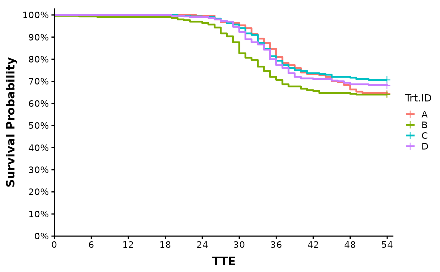
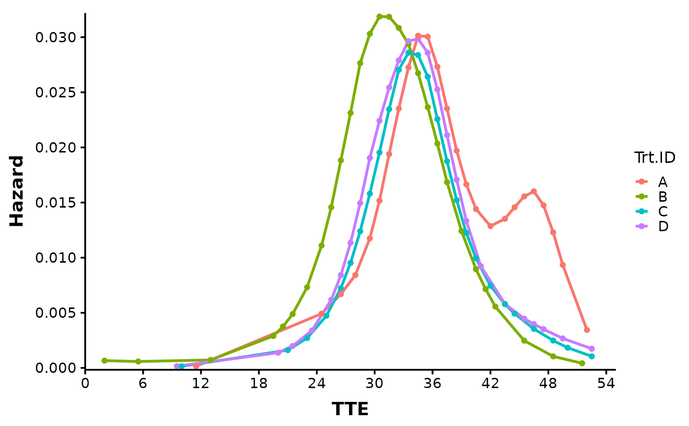
Surv_Plots(surv_db = surv_dat,
plot_prefix = "QCATC777",
xlab = "TTE",
plot = "both",
dailybin = FALSE,
theme = "publication")
#> $Survival_Plot
 #>
#> $Hazard_Plot
#>
#> $Hazard_Plot
 #>
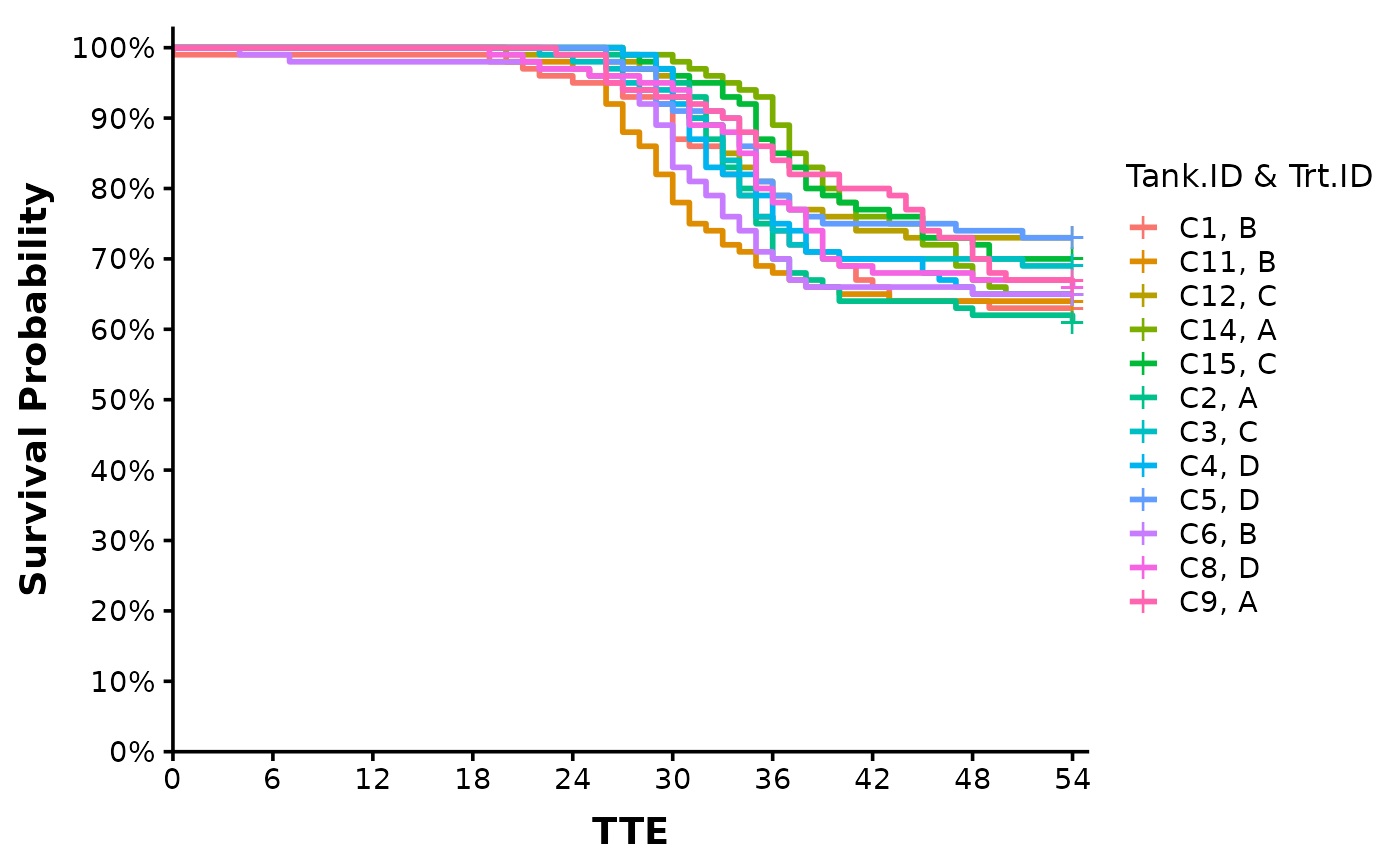
# If we want a plot for each tank, we can specify "Tank.ID" in the factor argument:
Surv_Plots(surv_db = surv_dat,
factor = "Tank.ID * Trt.ID",
plot_prefix = "QCATC777",
xlab = "TTE",
plot = "surv",
dailybin = FALSE,
theme = "publication")
#>
# If we want a plot for each tank, we can specify "Tank.ID" in the factor argument:
Surv_Plots(surv_db = surv_dat,
factor = "Tank.ID * Trt.ID",
plot_prefix = "QCATC777",
xlab = "TTE",
plot = "surv",
dailybin = FALSE,
theme = "publication")
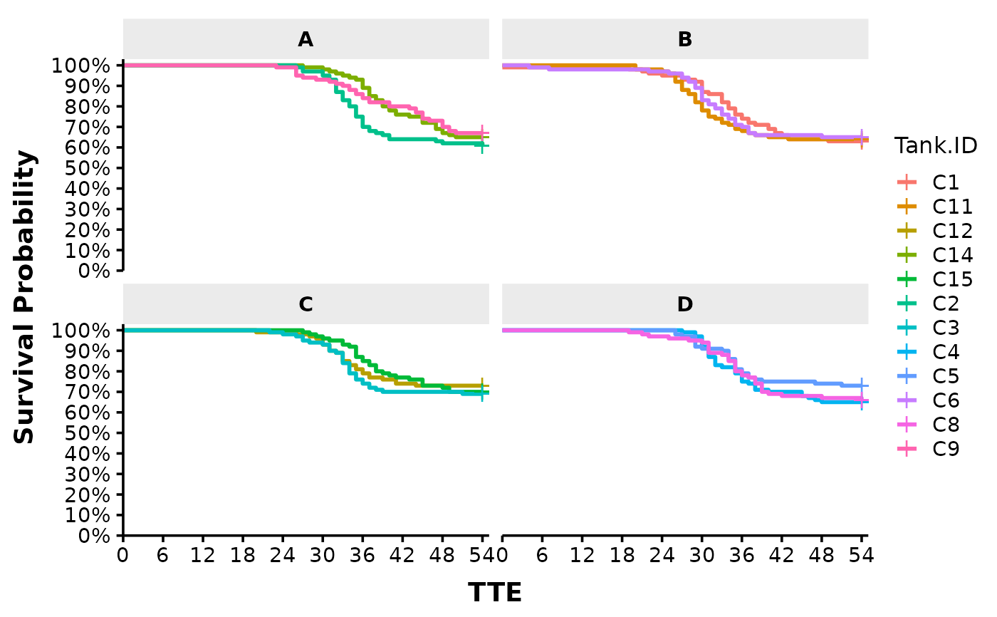
 # Plot each tank faceted by Trt.ID by changing "*" into "|" in the factor argument:
Surv_Plots(surv_db = surv_dat,
factor = "Tank.ID | Trt.ID",
plot_prefix = "QCATC777",
xlab = "TTE",
plot = "surv",
dailybin = FALSE,
theme = "publication")
# Plot each tank faceted by Trt.ID by changing "*" into "|" in the factor argument:
Surv_Plots(surv_db = surv_dat,
factor = "Tank.ID | Trt.ID",
plot_prefix = "QCATC777",
xlab = "TTE",
plot = "surv",
dailybin = FALSE,
theme = "publication")
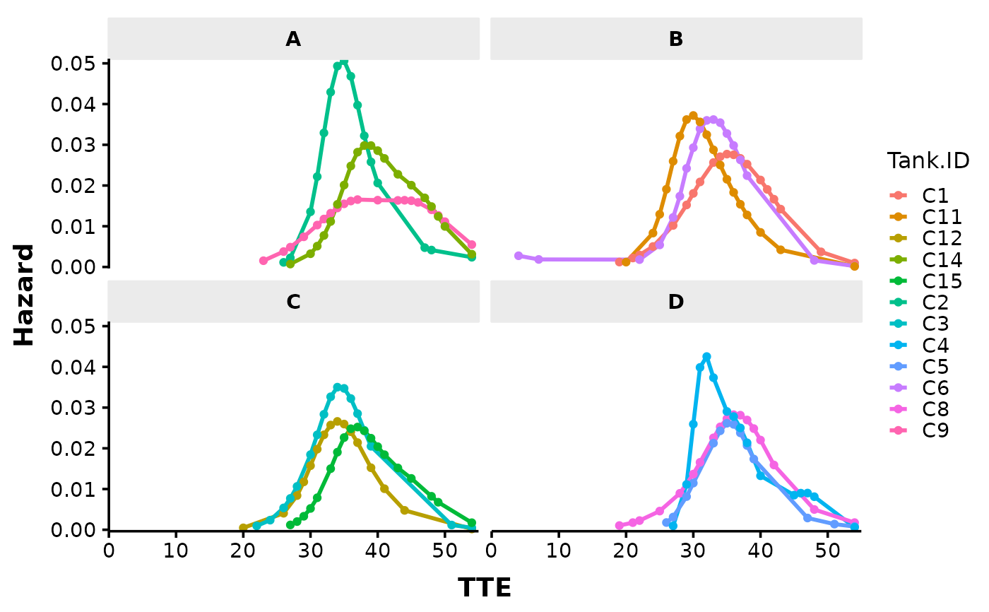
 # Tank specific hazard curves can also be created. The paramater phi often has to be
# specified for accurate estimation of the hazard curve of low sample size or single
# tank data. A phi between 1 to 2 is recommended based on estimates from past data
# with larger sample sizes. More info on estimation parameters can be found in the
# Details and Arguments section of the Surv_Plot() documentation.
Surv_Plots(surv_db = surv_dat,
factor = "Tank.ID | Trt.ID",
plot_prefix = "QCATC777",
phi = 1.5,
xlab = "TTE",
xbreaks = 10,
plot = "haz",
dailybin = FALSE,
theme = "publication")
#> Warning: Stop time must be > start time, NA created
# Tank specific hazard curves can also be created. The paramater phi often has to be
# specified for accurate estimation of the hazard curve of low sample size or single
# tank data. A phi between 1 to 2 is recommended based on estimates from past data
# with larger sample sizes. More info on estimation parameters can be found in the
# Details and Arguments section of the Surv_Plot() documentation.
Surv_Plots(surv_db = surv_dat,
factor = "Tank.ID | Trt.ID",
plot_prefix = "QCATC777",
phi = 1.5,
xlab = "TTE",
xbreaks = 10,
plot = "haz",
dailybin = FALSE,
theme = "publication")
#> Warning: Stop time must be > start time, NA created